Python Kriging in 2026: GSTools vs PyKrige vs SciKit-GStat Compared

You have 380 soil-moisture readings scattered across a 40-hectare field, and your boss wants a continuous surface, not dots. Inverse-distance weighting is the obvious first try — and it will quietly invent gradients that do not exist, because it has no concept of spatial correlation. Kriging does: it derives the weights from the data’s own variogram, returns a variance estimate alongside every prediction, and is the only interpolator in this class that is a best linear unbiased predictor.

The catch is that “kriging in Python” means three different libraries with three different philosophies. GSTools treats kriging as one feature of a full geostatistical toolbox. PyKrige is a focused kriging engine with a scikit-learn-compatible wrapper. SciKit-GStat is a variogram-analysis laboratory that happens to ship an ordinary kriging class. Picking the wrong one costs you a week of fighting an API that does not think the way your problem does.

The Short Version (TL;DR)

• Need random field simulation, global lat/lon support, or 3D meshes you can push into ParaView? Use GSTools — it is the only one of the three with first-class random field generation, rotation/anisotropy handling, and VTK export.
• Need an ordinary or universal kriging map from scattered points today, ideally inside a scikit-learn pipeline? Use PyKrige — a 10-line path from data to grid, plus a Krige wrapper that behaves like any scikit-learn estimator.
• Need to actually trust your variogram — comparing estimators, directional variograms, maximum-likelihood fitting? Use SciKit-GStat — roughly two dozen semivariance estimators and MLE fitting that the other two do not offer.
• If you must pick exactly one for production interpolation work: GSTools. It is the most actively maintained (last commit October 2026), and its covariance-model objects are reused across simulation, estimation, and kriging rather than being an afterthought.

Feature Comparison at a Glance

All figures pulled live from GitHub at publish time.

Which Library for Which Job

GSTools: A Geostatistical Toolbox, Not Just a Kriging Function

GSTools (655 stars, LGPL-3.0) models spatial structure with covariance model objects — Gaussian, Exponential, Stable, Matern and friends — that you can rotate, anisotropise, and reuse. The same model object drives random field generation, variogram fitting, and the kriging engine, which is why it wins on consistency.

The idiomatic workflow starts by estimating and fitting a variogram:

 1
 2
 3
 4
 5
 6
 7
 8
 9
10
11
12
13
14
15
16
17
18
19

import numpy as np
import gstools as gs

# generate a synthetic field with an exponential model
x = np.random.RandomState(19970221).rand(1000) * 100.
y = np.random.RandomState(20011012).rand(1000) * 100.
model = gs.Exponential(dim=2, var=2, len_scale=8)
srf = gs.SRF(model, mean=0, seed=19970221)
field = srf((x, y))

# estimate the variogram of the field
bin_center, gamma = gs.vario_estimate((x, y), field)

# fit the variogram with a stable model (no nugget fitted)
fit_model = gs.Stable(dim=2)
fit_model.fit_variogram(bin_center, gamma, nugget=False)
ax = fit_model.plot(x_max=max(bin_center))
ax.scatter(bin_center, gamma)
print(fit_model)

From there, kriging is a two-line step using the fitted model and your observations. Anisotropy is expressed directly on the model, which is far clearer than post-hoc axis scaling:

1
2
3

model = gs.Gaussian(dim=3, len_scale=[16, 8, 4], angles=(0.8, 0.4, 0.2))
krig = gs.krige.Ordinary(model, cond_pos=(x, y, z), cond_val=values)
field, variance = krig((grid_x, grid_y, grid_z))

Two capabilities matter in practice and are absent elsewhere in this comparison. First, conditioned simulation: srf can take observed points and produce realisations that honour them, which is what turns a single interpolated map into a defensible uncertainty study. Second, export: 3D fields go out through vtk_export() or to_pyvista(), so geologists and hydrologists can open them in the same viewer they already use.

PyKrige: The Fast Path From Points to Grid

PyKrige (862 stars, BSD-3-Clause) does one job and does it with minimal ceremony. Its classes map to classical geostatistics vocabulary: OrdinaryKriging, UniversalKriging, OrdinaryKriging3D, UniversalKriging3D, and RegressionKriging.

 1
 2
 3
 4
 5
 6
 7
 8
 9
10
11
12
13
14
15
16
17
18
19
20
21

import numpy as np
from pykrige.ok import OrdinaryKriging

data = np.array([
    [0.3, 1.2, 0.47],
    [1.9, 0.6, 0.56],
    [1.1, 3.2, 0.74],
    [3.3, 4.4, 1.47],
    [4.7, 3.8, 1.74],
])

gridx = np.arange(0.0, 5.5, 0.5)
gridy = np.arange(0.0, 5.5, 0.5)

OK = OrdinaryKriging(
    data[:, 0], data[:, 1], data[:, 2],
    variogram_model="linear",
    verbose=False,
    enable_plotting=False,
)
z, ss = OK.execute("grid", gridx, gridy)

Note what you get back: z is the interpolated surface, ss is the kriging variance grid. If you only read the first return value, you are throwing away the most valuable half of the output. Kriging variance is your map of “trust me here, doubt me there” — plot it before you ever publish an interpolated surface.

The scikit-learn bridge is the feature that converts PyKrige from a script into a pipeline component:

1
2
3
4
5

from pykrige.compat import Krige

krige = Krige(variogram_model="spherical", nlags=6, weight=True)
krige.fit(X_train, y_train)
predictions = krige.predict(X_test)

Because it obeys fit/predict, it drops into Pipeline, cross_val_score, and GridSearchCV alongside your other estimators. That is a genuinely rare property among geostatistics libraries, and it is the main reason to choose PyKrige over GSTools when your kriging is one step inside a larger modelling workflow.

Trade-off to accept: PyKrige’s last repository activity visible at publish time is October 2025, while GSTools and SciKit-GStat both saw commits in September/October 2026. It is stable, not abandoned — but if you need a new feature merged quickly, that matters.

SciKit-GStat: When the Variogram Is the Deliverable

SciKit-GStat (252 stars, MIT) inverts the usual priority. Its Variogram class is the centre of gravity, and the kriging class exists to consume a variogram you have already scrutinised.

 1
 2
 3
 4
 5
 6
 7
 8
 9
10
11

import skgstat as skg

coords, values = skg.data.meuse()          # bundled sample dataset
V = skg.Variogram(coords, values, model="spherical", n_lags=25, maxlag=1000)
print(V.parameters)                        # [sill, range, nugget]

# compare a robust estimator instead of the default Matheron estimator
V_cressie = skg.Variogram(coords, values, estimator="cressie", model="spherical")

ok = skg.OrdinaryKriging(V, min_points=2, max_points=10, mode="exact")
grid = ok.transform(gridx.ravel(), gridy.ravel())

The estimator argument is the reason this library exists. Robust estimators such as Cressie-Hawkins or Dowd down-weight outlier pairs, which changes the fitted range and sill — and therefore changes every downstream prediction. With n_lags, maxlag, bin_func, and directional support you can also see whether the variogram is isotropic; a directional variogram that diverges from the omnidirectional one is the single most common reason a kriged map looks “wrong” to a domain expert.

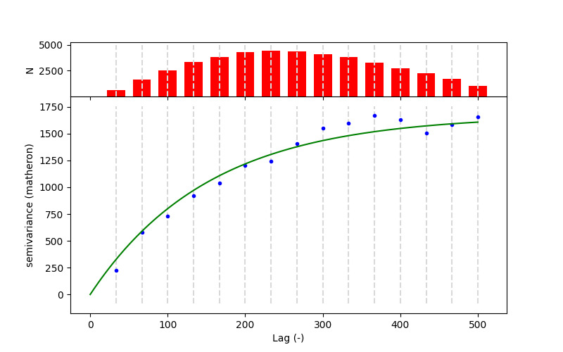
SciKit-GStat also offers maximum-likelihood variogram fitting, which avoids the subjective lag-binning step entirely. Lag binning is a modelling choice disguised as a preprocessing detail: change n_lags from 15 to 30 and the fitted range can move by 20 per cent.

The cost of this rigour: the API is scientific rather than ergonomic, the transform() pattern is unlike anything in scikit-learn, and star count is the lowest of the three. If you want one function that returns a map, this is not it.

Installing All Three Side by Side

All three coexist happily in one environment; they share only NumPy as a hard requirement. Conda users should prefer the conda-forge channel for binary dependency management.

1
2
3
4
5

# pip, from the official package indexes
pip install gstools pykrige scikit-gstat

# conda-forge equivalents
conda install -c conda-forge gstools pykrige scikit-gstat

For a reproducible analysis container, pin the interpreter and the three libraries on top of the official Python image:

 1
 2
 3
 4
 5
 6
 7
 8
 9
10

# docker-compose.yml — reproducible geostatistics sandbox
services:
  geo:
    image: python:3.12-slim
    working_dir: /work
    volumes:
      - ./:/work
    command: >
      bash -lc "pip install --no-cache-dir gstools==1.6 pykrige scikit-gstat &&
      python analyse.py"

Run docker compose run --rm geo python -c "import gstools, pykrige, skgstat" once to confirm all three imports resolve before you start an overnight batch job. Nothing wastes more compute than a 90-minute interpolation run that dies on the last import.

Where Teams Get Burned

• Ignoring the nugget effect. A nonzero nugget means short-range variability your sampling cannot resolve. Force the fit through the origin and you get an interpolator that is confidently wrong at every data point.
• Mixing units between coordinates and len_scale. The range parameter lives in the same units as your coordinates. Feed metres into a model fitted in feet and you have scaled your spatial structure by 3.28× without an error message.
• Binning choices pretending to be objective. n_lags and maxlag are model parameters, not settings. Report them, and test sensitivity.
• Forgetting cubic cost. Solving the kriging system is O(n³) in the number of conditioning points. Thousands of samples are fine; tens of thousands want a local neighbourhood — SciKit-GStat’s max_points and PyKrige’s nearest-neighbour kriging options exist precisely for this. Check your installed version’s argument names before assuming a parameter exists.
• Variogram fitted on the evaluation data. If you tune the variogram on all observations and then cross-validate on the same set, your error metrics are optimistic. Fit inside each fold.
• Duplicate or co-located samples. Two observations at identical coordinates make the kriging matrix singular. Deduplicate and average, or let the implementation handle exact values explicitly.
• Projecting lat/lon to a flat plane without thinking. For global datasets use GSTools’ geographic mode with metric scaling; for regional work, project to a metric CRS first — kriging weights are distance-based, and degrees are not distances.

Why Run Kriging on Your Own Hardware

Geostatistics work is unusually well suited to local execution, and that is not a small point in 2026. Field data — soil chemistry, groundwater levels, ore grades, air-quality sensor logs — is often commercially or legally sensitive, and pushing it into a hosted notebook platform is a data-governance decision, not a technical one. All three libraries are pure Python with NumPy underneath, install from a public index, and run offline once the wheels are cached. That means the entire pipeline — variogram fitting, cross-validation, simulation ensembles — can live on a laptop, a lab workstation, or a container on your own infrastructure with no external calls.

If you already run a geospatial stack, the practical complement to these libraries is a spatial database and a tile server: our guide to Python geospatial libraries covers the vector and raster side, and geophysical inversion tools shows how kriged surfaces feed forward modelling. For publishing the resulting maps, the scientific data visualization stacks guide covers the ParaView and VTK.js route that GSTools’ exporters target directly.

FAQ

Which Python library is best for kriging in 2026?

There is no single winner. Choose GSTools for random field simulation, geographic coordinates, 3D meshes, and the most active maintenance record. Choose PyKrige for the fastest path to an ordinary or universal kriging map and for scikit-learn pipeline integration. Choose SciKit-GStat when the variogram itself is the deliverable and you need robust estimators or maximum-likelihood fitting. Many production workflows use GSTools and SciKit-GStat together: SciKit-GStat to understand the variogram, GSTools to simulate and krige.

Is kriging better than inverse distance weighting?

For spatially correlated data, yes — kriging weights come from the fitted variogram rather than an arbitrary inverse-power rule, and kriging also returns a prediction variance. Inverse distance weighting cannot tell you where it is uncertain and will smooth away real structure. The trade-off is that kriging requires you to model spatial structure, which is exactly the step inverse distance weighting avoids.

Does PyKrige work with scikit-learn?

Yes, through pykrige.compat.Krige, which implements fit and predict and can therefore be used inside Pipeline, cross_val_score, and GridSearchCV. This compatibility wrapper is the main advantage PyKrige holds over GSTools for teams whose modelling code is already organised around scikit-learn.

Can these libraries handle 3D and time-space data?

GSTools and PyKrige both ship 3D kriging classes, and GSTools also models space-time covariance with anisotropic length scales. SciKit-GStat is primarily a 2D/3D distance tool focused on variogram estimation rather than high-dimensional production kriging. For volumes that must be inspected visually, GSTools’ VTK and PyVista export is the most direct route into ParaView.

How many data points can kriging handle?

Practical limits come from the O(n³) solve rather than any library restriction. Tens of thousands of conditioning points become slow and memory-hungry, so production setups typically switch to a moving neighbourhood — a limited number of nearest conditioning points per prediction location. SciKit-GStat exposes this through max_points, and PyKrige offers nearest-neighbour kriging variants; always confirm the exact argument name for your installed version.

Do I need a GPU to run kriging?

No. These libraries are CPU-bound NumPy implementations, and the bottleneck is the linear solve, not matrix arithmetic that vectorises well. For ensemble simulation, run realisations as parallel processes across CPU cores instead of reaching for a GPU.

💰 想测试你的市场判断力？我用 Polymarket 做预测市场交易——这是全球最大的预测市场平台，从大选结果到技术监管时间线，什么都可以押注。和赌博不同，这是真正的信息市场：你懂的信息越多，胜率越高。我靠预测技术相关事件的走向已经赚了不少。用我的邀请链接注册：Polymarket.com